# Map projections are nonlinear transforms (λ,φ) -> (x,y)
#	where	λ = longitude	φ = latitude

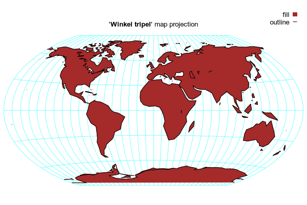
# "Winkel tripel" map projection (Oswald Winkel 1874-1953)
# This is the arithmetic mean of an equirectangular projection and the
# Aitoff projection.

# Note: mouse tracking does not correctly report longitude, latitude
unset mouse

set title "'{/:Bold Winkel tripel}' map projection"

π = pi
φ1 = acos(2./π)
sinc(x) = (x==0) ? 1.0 : sin(x) / x
α(λ,φ) = acos(cos(φ) * cos(λ/2.))
x_W3(λ, φ) = 0.5 * (λ*cos(φ1) + (2*cos(φ)*sin(λ/2.))/sinc(α(λ,φ)))
y_W3(λ, φ) = 0.5 * (φ + sin(φ)/sinc(α(λ,φ)))

set key top right at screen 0.98, 0.95 samplen 0.3
set angle degrees
unset xtics
unset ytics
unset border
set lmargin 1
set rmargin 1
set size ratio 0.5

set xrange [-180:180]
set yrange [-90:90]

plot for [λ=-180:180:10] [φ=-90:90] '+' using (x_W3(λ,φ)):(y_W3(λ,φ)) with lines lc "cyan" lw .5 notitle, \
     for [φ = -90:90:30] [λ=-180:180:10] '+' using (x_W3(λ,φ)):(y_W3(λ,φ)) with lines lc "cyan" lw .5 notitle, \
     'world.dat' using (x_W3($1,$2)):(y_W3($1,$2)) with filledcurve fc "brown" title "fill", \
     'world.dat' using (x_W3($1,$2)):(y_W3($1,$2)) with lines lc "black" title "outline"


Click here for minimal script to generate this plot

#
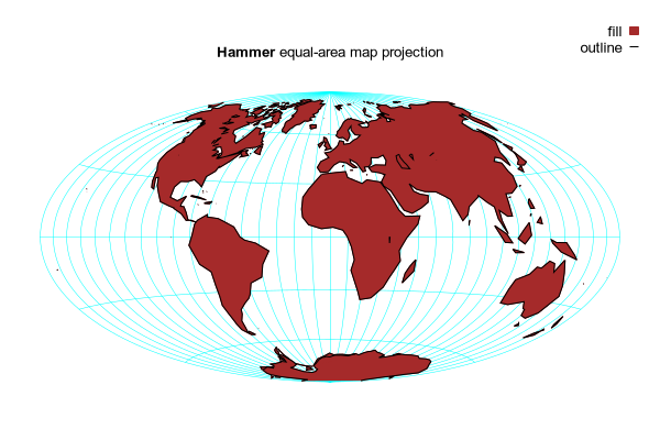
# Hammer equal-area projection (Ernst Hammer 1892)
#

set title "{/:Bold Hammer} equal-area map projection"

x_Hammer(λ, φ) = (2*sqrt(2)*cos(φ)*sin(λ/2)) / sqrt(1.0 + cos(φ)*cos(λ/2))
y_Hammer(λ, φ) = sqrt(2)*sin(φ) / sqrt(1.0 + cos(φ)*cos(λ/2))

# Note: To have mouse tracking report coordinates that correspond to the
# map projection, we must define an inverse function dependent on both
# screen x and screen y.
#
Z(x,y) = sqrt( 1.0 - (x/4)**2 - (y/2)**2 )
lon(x,y) = 2. * atan( x*Z(x,y) / (4*Z(x,y)**2 - 2) )
lat(x,y) = asin(Z(x,y)*y)
set mouse mouseformat function sprintf("Longitude %.2f Latitude %.2f", lon(x,y), lat(x,y))

set xrange [-π : π]
set yrange [-π/2 : π/2]

plot for [λ=-180:180:10] [φ=-90:90] '+' using (x_Hammer(λ,φ)):(y_Hammer(λ,φ)) with lines lc "cyan" lw .5 notitle, \
     for [φ = -90:90:30] [λ=-180:180:10] '+' using (x_Hammer(λ,φ)):(y_Hammer(λ,φ)) with lines lc "cyan" lw .5 notitle, \
     'world.dat' using (x_Hammer($1,$2)):(y_Hammer($1,$2)) with filledcurve fc "brown" title "fill", \
     'world.dat' using (x_Hammer($1,$2)):(y_Hammer($1,$2)) with lines lc "black" title "outline"


Click here for minimal script to generate this plot

#
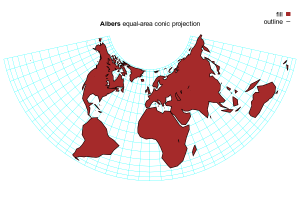
# Albers equal-area conic projection
# Heinrich C. Albers 1805
#

set title "{/:Bold Albers} equal-area conic projection"

set auto
φ0 = 0.
φ1 = 0.
φ2 = 60.
λ0 = 0.
n = 0.5 * (sin(φ1) + sin(φ2))
θ(λ) = n*(λ-λ0)
C = cos(φ1)**2 + 2*n*sin(φ1)
ρ(φ) = sqrt(C - 2*n*sin(φ)) / n
ρ0 = ρ(φ0)

x_Albers(λ, φ) = ρ(φ) * sin(θ(λ))
y_Albers(λ, φ) = ρ0 - ρ(φ)*cos(θ(λ))

clip(south) = south < -60. ? NaN : south

#
# inverse functions for map readout
#
lon(x,y) = atan( x/(ρ0-y) ) / n
lat(x,y) = asin( (C - n*n*(x**2 + (ρ0-y)**2)) / (2*n) )
mouse_readout(x,y) = sprintf("Longitude %.2f Latitude %.2f", lon(x,y), lat(x,y))
set mouse mouseformat function mouse_readout(x,y)

plot for [λ=-180:180:10] [φ=-60:90] '+' using (x_Albers(λ,φ)):(y_Albers(λ,φ)) with lines lc "cyan" lw .5 notitle, \
     for [φ = -60:90:10] [λ=-180:180:10] '+' using (x_Albers(λ,φ)):(y_Albers(λ,φ)) with lines lc "cyan" lw .5 notitle, \
     'world.dat' using (x_Albers($1,clip($2))):(y_Albers($1,clip($2))) with filledcurve fc "brown" title "fill", \
     'world.dat' using (x_Albers($1,clip($2))):(y_Albers($1,clip($2))) with lines lc "black" title "outline"


Click here for minimal script to generate this plot

# return mouse readout to default state
set mouse mouseformat 0