#
# $Id: airfoil.dem,v 1.10 2006/06/30 02:17:21 sfeam Exp $
#
# This demo shows how to use bezier splines to define NACA four
# series airfoils and complex variables to define Joukowski
# Airfoils.  It will be expanded after overplotting in implemented
# to plot Coefficient of Pressure as well.
#		Alex Woo, Dec. 1992
#
# The definitions below follows: "Bezier presentation of airfoils",
# by Wolfgang Boehm, Computer Aided Geometric Design 4 (1987) pp 17-22.
#
#				Gershon Elber, Nov. 1992
#
# m = percent camber
# p = percent chord with maximum camber
print  "NACA four series airfoils by bezier splines"
print  "Will add pressure distribution later with Overplotting"
mm = 0.6
# NACA6xxx
thick = 0.09
# nine percent  NACAxx09
pp = 0.4
# NACAx4xx
# Combined this implies NACA6409 airfoil
#
# Airfoil thickness function.
#
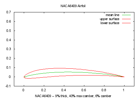
set xlabel "NACA6409 -- 9% thick, 40% max camber, 6% camber"
x0 = 0.0
y0 = 0.0
x1 = 0.0
y1 = 0.18556
x2 = 0.03571
y2 = 0.34863
x3 = 0.10714
y3 = 0.48919
x4 = 0.21429
y4 = 0.58214
x5 = 0.35714
y5 = 0.55724
x6 = 0.53571
y6 = 0.44992
x7 = 0.75000
y7 = 0.30281
x8 = 1.00000
y8 = 0.01050
#
# Directly defining the order 8 Bezier basis function for a faster evaluation.
#
bez_d4_i0(x) =     (1 - x)**4
bez_d4_i1(x) = 4 * (1 - x)**3 * x
bez_d4_i2(x) = 6 * (1 - x)**2 * x**2
bez_d4_i3(x) = 4 * (1 - x)**1 * x**3
bez_d4_i4(x) =                  x**4

bez_d8_i0(x) =      (1 - x)**8
bez_d8_i1(x) =  8 * (1 - x)**7 * x
bez_d8_i2(x) = 28 * (1 - x)**6 * x**2
bez_d8_i3(x) = 56 * (1 - x)**5 * x**3
bez_d8_i4(x) = 70 * (1 - x)**4 * x**4
bez_d8_i5(x) = 56 * (1 - x)**3 * x**5
bez_d8_i6(x) = 28 * (1 - x)**2 * x**6
bez_d8_i7(x) =  8 * (1 - x)    * x**7
bez_d8_i8(x) =                   x**8


m0 = 0.0
m1 = 0.1
m2 = 0.1
m3 = 0.1
m4 = 0.0
mean_y(t) = m0 * mm * bez_d4_i0(t) + \
	    m1 * mm * bez_d4_i1(t) + \
	    m2 * mm * bez_d4_i2(t) + \
	    m3 * mm * bez_d4_i3(t) + \
	    m4 * mm * bez_d4_i4(t)

p0 = 0.0
p1 = pp / 2
p2 = pp
p3 = (pp + 1) / 2
p4 = 1.0
mean_x(t) = p0 * bez_d4_i0(t) + \
	    p1 * bez_d4_i1(t) + \
	    p2 * bez_d4_i2(t) + \
	    p3 * bez_d4_i3(t) + \
	    p4 * bez_d4_i4(t)

z_x(x) = x0 * bez_d8_i0(x) + x1 * bez_d8_i1(x) + x2 * bez_d8_i2(x) + \
	 x3 * bez_d8_i3(x) + x4 * bez_d8_i4(x) + x5 * bez_d8_i5(x) + \
	 x6 * bez_d8_i6(x) + x7 * bez_d8_i7(x) + x8 * bez_d8_i8(x)

z_y(x, tk) = \
   y0 * tk * bez_d8_i0(x) + y1 * tk * bez_d8_i1(x) + y2 * tk * bez_d8_i2(x) + \
   y3 * tk * bez_d8_i3(x) + y4 * tk * bez_d8_i4(x) + y5 * tk * bez_d8_i5(x) + \
   y6 * tk * bez_d8_i6(x) + y7 * tk * bez_d8_i7(x) + y8 * tk * bez_d8_i8(x)

#
# Given t value between zero and one, the airfoild curve is defined as
#
#			c(t) = mean(t1(t)) +/- z(t2(t)) n(t1(t)),
#
# where n is the unit normal to the mean line. See the above paper for more.
#
# Unfortunately, the parametrization of c(t) is not the same for mean(t1)
# and z(t2). The mean line (and its normal) can assume linear function t1 = t,
#                                                     -1
# but the thickness z_y is, in fact, a function of z_x  (t). Since it is
# not obvious how to compute this inverse function analytically, we instead
# replace t in c(t) equation above by z_x(t) to get:
#
#			c(z_x(t)) = mean(z_x(t)) +/- z(t) n(z_x(t)),
#
# and compute and display this instead. Note we also ignore n(t) and assumes
# n(t) is constant in the y direction,
#

airfoil_y1(t, thick) = mean_y(z_x(t)) + z_y(t, thick)
airfoil_y2(t, thick) = mean_y(z_x(t)) - z_y(t, thick)
airfoil_y(t) = mean_y(z_x(t))
airfoil_x(t) = mean_x(z_x(t))
unset grid
unset zeroaxis
set parametric
set xrange [-0.1:1.1]
set yrange [-0.1:.7]
set trange [ 0.0:1.0]
set title "NACA6409 Airfoil"
plot airfoil_x(t), airfoil_y(t) title "mean line" w l lt 2, \
     airfoil_x(t), airfoil_y1(t, thick) title "upper surface" w l lt 1, \
     airfoil_x(t), airfoil_y2(t, thick) title "lower surface" w l lt 1

Click here for minimal script to generate this plot


