#
# $Id: prob.dem,v 1.9 2006/06/14 03:24:09 sfeam Exp $
#
# Demo Statistical Functions version 2.3
#
# Copyright (c) 1991, 1992 Jos van der Woude, jvdwoude@hut.nl

# History:
#    -- --- 1992 Jos van der Woude:  1st version
#    06 Jun 2006 Dan Sebald:  Added some variety and plotting techniques for
#                             better visual effect.  More tutorial in nature.

print "                   Statistical Library Demo, version 2.3"
print "\n          Copyright (c) 1991, 1992, Jos van de Woude, jvdwoude@hut.nl"
print "\n\n\n\n\n\n\n"
print "NOTE: contains 54 plots and consequently takes a lot of time to run"
print "                      Press Ctrl-C to exit right now"

Click here for minimal script to generate this plot

load "stat.inc"

eps = 1.0e-10  # Supposed to be float resolution (nice if were defined internally)

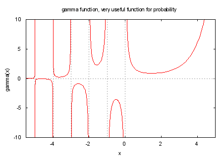
## Gamma function
xmin = -5.5
xmax = 5
ymin = -10
ymax = 10
unset key
set xzeroaxis
gsampfunc(t,n) = t<0?0.5*1/(-t+1.0)**n:1.0-0.5*1/(t+1.0)**n
set parametric
set trange [-1:1]
set sample 200
set xrange [xmin : xmax]
set yrange [ymin : ymax]
set xlabel "x"
set ylabel "gamma(x)"
set arrow 1 from  0,ymin to  0,ymax nohead lt 0
set arrow 2 from -1,ymin to -1,ymax nohead lt 0
set arrow 3 from -2,ymin to -2,ymax nohead lt 0
set arrow 4 from -3,ymin to -3,ymax nohead lt 0
set arrow 5 from -4,ymin to -4,ymax nohead lt 0
set arrow 6 from -5,ymin to -5,ymax nohead lt 0
set title "gamma function, very useful function for probability"
plot gsampfunc(5*t,5)-6, gamma(gsampfunc(5*t,5)-6) lt 1, \
     gsampfunc(5*t,5)-5, gamma(gsampfunc(5*t,5)-5) lt 1, \
     gsampfunc(5*t,4)-4, gamma(gsampfunc(5*t,4)-4) lt 1, \
     gsampfunc(5*t,3)-3, gamma(gsampfunc(5*t,3)-3) lt 1, \
     gsampfunc(5*t,2)-2, gamma(gsampfunc(5*t,2)-2) lt 1, \
     gsampfunc(5*t,1)-1, gamma(gsampfunc(5*t,1)-1) lt 1, \
     5*gsampfunc(5*t,2), gamma(5*gsampfunc(5*t,2)) lt 1

Click here for minimal script to generate this plot

ymin = ymin/2
ymax = ymax/2
set yrange [ymin:ymax]
set ylabel "lgamma(x)"
set arrow 1 from  0,ymin to  0,ymax nohead lt 0
set arrow 2 from -1,ymin to -1,ymax nohead lt 0
set arrow 3 from -2,ymin to -2,ymax nohead lt 0
set arrow 4 from -3,ymin to -3,ymax nohead lt 0
set arrow 5 from -4,ymin to -4,ymax nohead lt 0
set arrow 6 from -5,ymin to -5,ymax nohead lt 0
set title "log gamma function, similarly very useful function"
plot gsampfunc(5*t,5)-6, lgamma(gsampfunc(5*t,5)-6) lt 1, \
     gsampfunc(5*t,5)-5, lgamma(gsampfunc(5*t,5)-5) lt 1, \
     gsampfunc(5*t,4)-4, lgamma(gsampfunc(5*t,4)-4) lt 1, \
     gsampfunc(5*t,3)-3, lgamma(gsampfunc(5*t,3)-3) lt 1, \
     gsampfunc(5*t,3)-2, lgamma(gsampfunc(5*t,3)-2) lt 1, \
     gsampfunc(5*t,3)-1, lgamma(gsampfunc(5*t,3)-1) lt 1, \
     5*gsampfunc(5*t,3), lgamma(5*gsampfunc(5*t,3)) lt 1

Click here for minimal script to generate this plot

# Arcsinus PDF and CDF
r = 2.0
mu = 0.0
sigma = r / sqrt2
xmin = -(r+1)
xmax = r+1
unset key
set zeroaxis
set xrange [xmin : xmax]
set yrange [-0.2 : 1.2]
set xlabel "x ->"
set ylabel "probability density ->"
set xtics autofreq
set ytics autofreq
set format x "%.1f"
set format y "%.1f"
set sample 50*xmax+1
set title "arcsin PDF with r = 2.0"
plot arcsin(x, r)

Click here for minimal script to generate this plot

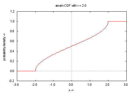
set title "arcsin CDF with r = 2.0"
set yrange [-0.2 : 1.2]
plot carcsin(x, r)

Click here for minimal script to generate this plot

# Beta PDF and CDF
p = 5.0; q = 3.0
mu = p / (p + q)
sigma = sqrt(p**q) / ((p + q ) * sqrt(p + q + 1.0))
xmin = 0.0
xmax = 1.0
#Mode of beta PDF used
ymax = (p < 1.0 || q < 1.0) ? 2.0 : 1.4 * beta((p - 1.0)/(p + q - 2.0), p, q)
set key right box
set zeroaxis
set xrange [xmin : xmax]
set yrange [0 : ymax]
set xlabel "x ->"
set ylabel "probability density ->"
set xtics autofreq
set ytics autofreq
set format x "%.1f"
set format y "%.1f"
set sample 200
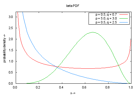
set title "beta PDF"
plot beta(x, 0.5, 0.7) title "p = 0.5, q = 0.7", \
     beta(x, 5.0, 3.0) title "p = 5.0, q = 3.0", \
     beta(x, 0.5, 2.5) title "p = 0.5, q = 2.5"

Click here for minimal script to generate this plot

set yrange [0:1.1]
set title "incomplete beta CDF"
set key left box
plot cbeta(x, 0.5, 0.7) title "p = 0.5, q = 0.7", \
     cbeta(x, 5.0, 3.0) title "p = 5.0, q = 3.0", \
     cbeta(x, 0.5, 2.5) title "p = 0.5, q = 2.5"

Click here for minimal script to generate this plot

# Binomial PDF and CDF
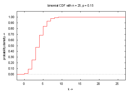
n = 25; p = 0.15
mu = n * p
sigma = sqrt(n * p * (1.0 - p))
xmin = int(mu - 4.0 * sigma)
xmin = xmin < -2 ? -2 : xmin
xmax = int(mu + 4.0 * sigma)
xmax = xmax < n+2 ? n+2 : xmax
ymax = 1.1 * binom(int((n+1)*p), n, p) #Mode of binomial PDF used
unset key
unset zeroaxis
set xrange [xmin : xmax]
set yrange [0 : ymax]
set xlabel "k ->"
set ylabel "probability density ->"
set ytics 0, ymax / 10, ymax
set format x "%2.0f"
set format y "%3.2f"
set sample (xmax - xmin) + 1
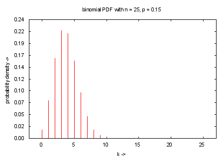
set title "binomial PDF with n = 25, p = 0.15"
plot binom(x, n, p) with impulses

Click here for minimal script to generate this plot

set ytics autofreq
set xzeroaxis
set title "binomial CDF with n = 25, p = 0.15"
set yrange [-0.1 : 1.1]
set ytics 0, 0.1, 1.0
plot cbinom(x, n, p) with steps

Click here for minimal script to generate this plot

# Cauchy PDF and CDF
a = 0.0; b = 2.0
#cauchy PDF has no moments
xmin = a - 5.0 * b
xmax = a + 5.0 * b
ymax = 1.1 * cauchy(a, a, b) #Mode of cauchy PDF used
set key left box
set zeroaxis
set xlabel "x ->"
set ylabel "probability density ->"
set xtics autofreq
set ytics autofreq
set format x "%.1f"
set format y "%.2f"
set sample 100
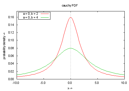
set title "cauchy PDF"
a=0
b=2
plot [xmin:xmax] [0:ymax] cauchy(x, 0, 2) title "a = 0, b = 2", \
                          cauchy(x, 0, 4) title "a = 0, b = 4"

Click here for minimal script to generate this plot

set title "cauchy CDF"
plot [xmin:xmax] [0:1.0] ccauchy(x, 0, 2) title "a = 0, b = 2", \
                         ccauchy(x, 0, 4) title "a = 0, b = 4"

Click here for minimal script to generate this plot

# Chi-square PDF and CDF
k = 4.0
mu = k
sigma = sqrt(2.0 * k)
xmin = mu - 4.0 * sigma
xmin = xmin < 0 ? 0 : xmin
xmax = int(mu + 4.0 * sigma)
k = 2.0
ymax = (k > 2.0 ? 1.1*chisq(k - 2.0, k) : 0.5) #Mode of chi PDF used
set key right box
set zeroaxis
set xrange [xmin+eps : xmax] #Discontinuity at zero for k < 2
set yrange [0:ymax]
set xlabel "x ->"
set ylabel "probability density ->"
set xtics autofreq
set ytics autofreq
set format x "%.1f"
set format y "%.2f"
set sample 100
set title "chi-square PDF"
set key right box
set samples 15*20+1
keystr(k) = sprintf("k = %d", k)
plot k = 1, x==0?1/0:chisq(x, k) title keystr(k), \
     k = 2, x==0?1/0:chisq(x, k) title keystr(k), \
     k = 3, chisq(x, k) title keystr(k), \
     k = 4, chisq(x, k) title keystr(k), \
     k = 5, chisq(x, k) title keystr(k), \
     k = 6, chisq(x, k) title keystr(k), \
     k = 7, chisq(x, k) title keystr(k), \
     k = 8, chisq(x, k) title keystr(k)

Click here for minimal script to generate this plot

set yrange [0:1.1]
set key bottom right box
set title "chi-square CDF"
plot k = 1, cchisq(x, k) title keystr(k), \
     k = 2, cchisq(x, k) title keystr(k), \
     k = 3, cchisq(x, k) title keystr(k), \
     k = 4, cchisq(x, k) title keystr(k), \
     k = 5, cchisq(x, k) title keystr(k), \
     k = 6, cchisq(x, k) title keystr(k), \
     k = 7, cchisq(x, k) title keystr(k), \
     k = 8, cchisq(x, k) title keystr(k)

Click here for minimal script to generate this plot

# Erlang PDF and CDF
lambda = 1.0; n = 2.0
mu = n / lambda
sigma = sqrt(n) / lambda
xmax = int(mu + 5.0 * sigma)
n = 1.0
ymax = n < 2.0 ? 1.0 : 1.1 * erlang((n - 1.0) / lambda, n, lambda) #Mode of erlang PDF used
set zeroaxis
set xlabel "x ->"
set ylabel "probability density ->"
set xtics autofreq
set ytics autofreq
set format x "%.1f"
set format y "%.1f"
set sample 100
set title "erlang PDF"
set key top right box
l1 = 1.0; l2 = 0.5
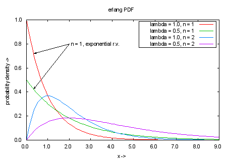
set arrow 1 from 2,0.8 to 0.33,erlang(0.33,1,l1)
set arrow 2 from 2,0.8 to 0.33,erlang(0.33,1,l2)
set label 1 "n = 1, exponential r.v." at 2.1,0.8 left
keystr(n,lambda) = sprintf("lambda = %0.1f, n = %d", lambda, n)
plot [0:xmax] [0:ymax] n = 1, lambda = l1, erlang(x, n, lambda) title keystr(n,lambda), \
                       n = 1, lambda = l2, erlang(x, n, lambda) title keystr(n,lambda), \
                       n = 2, lambda = l1, erlang(x, n, lambda) title keystr(n,lambda), \
                       n = 2, lambda = l2, erlang(x, n, lambda) title keystr(n,lambda)

Click here for minimal script to generate this plot

unset label 1
unset arrow 1; unset arrow 2
set title "erlang CDF"
set key bottom right box
plot [0:xmax] [0:1.1] n = 1, lambda = l1, cerlang(x, n, lambda) title keystr(n,lambda), \
                      n = 1, lambda = l2, cerlang(x, n, lambda) title keystr(n,lambda), \
                      n = 2, lambda = l1, cerlang(x, n, lambda) title keystr(n,lambda), \
                      n = 2, lambda = l2, cerlang(x, n, lambda) title keystr(n,lambda)

Click here for minimal script to generate this plot

# Thanks to mrb2j@kelvin.seas.Virginia.EDU for telling us about this.
# Extreme (Gumbel extreme value) PDF and CDF
alpha = 1.0; u = 0.0
mu = u + (0.577215665/alpha)   # Euler's constant
sigma = pi/(sqrt(6.0)*alpha)
xmin = mu - 6.0 * sigma
xmax = mu + 6.0 * sigma
ymax = 1.1 * extreme(u, u, alpha) #Mode of extreme PDF used
ymax = int(10*ymax)/10.0
set zeroaxis
set xlabel "x ->"
set ylabel "probability density ->"
set xtics autofreq
set ytics autofreq
set format x "%.1f"
set format y "%.2f"
set sample 100
set title "extreme PDF"
set key top left box
plot [xmin:xmax] [0:ymax] extreme(x, 1.0, 0.5) title "alpha = 0.5, u = 1.0", \
                          extreme(x, 0.0, 1.0) title "alpha = 1.0, u = 0.0"

Click here for minimal script to generate this plot

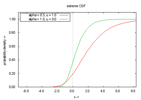
set title "extreme CDF"
plot [xmin:xmax] [0:1.1] cextreme(x, 1.0, 0.5) title "alpha = 0.5, u = 1.0", \
                         cextreme(x, 0.0, 1.0) title "alpha = 1.0, u = 0.0"

Click here for minimal script to generate this plot

# F PDF and CDF
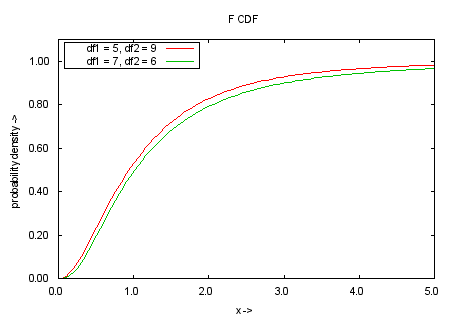
df1 = 5.0; df2 = 9.0
mu = df2 < 2.0 ? 1.0 : df2 / (df2 - 2.0)
sigma = df2 < 4.0 ? 1.0 : mu * sqrt(2.0 * (df1 + df2 - 2.0) / (df1 * (df2 - 4.0)))
xmin = mu - 3.0 * sigma
xmin = xmin < 0 ? 0 : xmin
xmax = int(mu + 3.0 * sigma)
#Mode of F PDF used
ymax = df1 < 3.0 ? 1.0 : 1.1 * f((df1 / 2.0 - 1.0) / (df1 / 2.0 + df1 / df2), df1, df2)
set zeroaxis
set xlabel "x ->"
set ylabel "probability density ->"
set xtics autofreq
set ytics autofreq
set format x "%.1f"
set format y "%.2f"
set sample 100
set title "F PDF"
set key right box
plot [xmin:xmax] [0:ymax] f(x, 5.0, 9.0) title "df1 = 5, df2 = 9", \
                          f(x, 7.0, 6.0) title "df1 = 7, df2 = 6"

Click here for minimal script to generate this plot

set title "F CDF"
set key left box
plot [xmin:xmax] [0:1.1] cf(x, 5.0, 9.0) title "df1 = 5, df2 = 9", \
                         cf(x, 7.0, 6.0) title "df1 = 7, df2 = 6"

Click here for minimal script to generate this plot

# Gamma PDF and incomplete gamma CDF
rho = 1.0; lambda = 1.3
mu = rho / lambda
sigma = sqrt(rho) / lambda
xmin = mu - 4.0 * sigma
xmin = xmin < 0 ? 0 : xmin
xmax = mu + 4.0 * sigma
ymax = rho < 1.0 ? 2.0 : 1.1 * gmm((rho - 1.0) / lambda, rho, lambda) #Mode of gamma pdf used
set zeroaxis
set xlabel "x ->"
set ylabel "probability density ->"
set xtics autofreq
set ytics autofreq
set format x "%.1f"
set format y "%.1f"
set sample 100
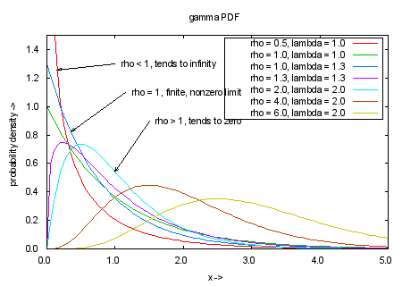
set title "gamma PDF"
set key right
r1 = 0.5; r2 = 1.0; r3 = 1.0; r4 = 1.3; r5 = 2.0; r6 = 4.0; r7 = 6.0
l1 = 1.0; l2 = 1.0; l3 = 1.3; l4 = 1.3; l5 = 2.0; l6 = 2.0; l7 = 2.0
set arrow 1 from 1,1.3 to 0.15,gmm(0.15,r1,l1)
set label 1 "rho < 1, tends to infinity" at 1.1,1.3 left
set arrow 2 from 1.15,1.1 to 0.35,gmm(0.35,r3,l3)
set label 2 "rho = 1, finite, nonzero limit" at 1.25,1.1 left
set arrow 3 from 1.5,0.9 to 1.0,gmm(1.0,r5,l5)
set label 3 "rho > 1, tends to zero" at 1.6,0.9 left
keystr(rho,lambda) = sprintf("rho = %0.1f, lambda = %0.1f", rho, lambda)
plot [0:5] [0:1.5] rho = r1, lambda = l1, gmm(x, rho, lambda) title keystr(rho,lambda), \
                   rho = r2, lambda = l2, gmm(x, rho, lambda) title keystr(rho,lambda), \
                   rho = r3, lambda = l3, gmm(x, rho, lambda) title keystr(rho,lambda), \
                   rho = r4, lambda = l4, gmm(x, rho, lambda) title keystr(rho,lambda), \
                   rho = r5, lambda = l5, gmm(x, rho, lambda) title keystr(rho,lambda), \
                   rho = r6, lambda = l6, gmm(x, rho, lambda) title keystr(rho,lambda), \
                   rho = r7, lambda = l7, gmm(x, rho, lambda) title keystr(rho,lambda)

Click here for minimal script to generate this plot

unset label 1; unset label 2; unset label 3
unset arrow 1; unset arrow 2; unset arrow 3
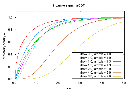
set title "incomplete gamma CDF"
set key right bottom
plot [0:5] [0:1.1] rho = r1, lambda = l1, cgmm(x, rho, lambda) title keystr(rho,lambda), \
                   rho = r2, lambda = l2, cgmm(x, rho, lambda) title keystr(rho,lambda), \
                   rho = r3, lambda = l3, cgmm(x, rho, lambda) title keystr(rho,lambda), \
                   rho = r4, lambda = l4, cgmm(x, rho, lambda) title keystr(rho,lambda), \
                   rho = r5, lambda = l5, cgmm(x, rho, lambda) title keystr(rho,lambda), \
                   rho = r6, lambda = l6, cgmm(x, rho, lambda) title keystr(rho,lambda), \
                   rho = r7, lambda = l7, cgmm(x, rho, lambda) title keystr(rho,lambda)

Click here for minimal script to generate this plot

# Geometric PDF and CDF
p = 0.4
mu = (1.0 - p) / p
sigma = sqrt(mu / p)
xmin = int(mu - 4.0 * sigma)
xmin = xmin < -1 ? -1 : xmin
xmin = -1
xmax = int(mu + 4.0 * sigma)
ymax = 1.1 * geometric(0, p) #mode of geometric PDF used
unset key
unset zeroaxis
set xrange [xmin : xmax]
set yrange [0 : ymax]
set xlabel "k ->"
set ylabel "probability density ->"
set ytics 0, ymax / 10, ymax
set format x "%2.0f"
set format y "%3.2f"
set sample (xmax - xmin) + 1
set title "geometric PDF with p = 0.4"
plot geometric(x, p) with impulses

Click here for minimal script to generate this plot

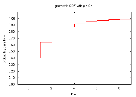
set title "geometric CDF with p = 0.4"
set yrange [0 : 1.1]
set ytics 0, 0.1, 1.0
plot cgeometric(x, p) with steps

Click here for minimal script to generate this plot

# Half normal PDF and CDF
mu = sqrt2invpi
sigma = 1.0
s = sigma*sqrt(1.0 - 2.0/pi)
xmin = -0.2
xmax = mu + 4.0 * s
ymax = 1.1 * halfnormal(0, sigma) #Mode of half normal PDF used
unset key
set zeroaxis
set xrange [xmin: xmax]
set yrange [-0.1: ymax]
set xlabel "x ->"
set ylabel "probability density ->"
set xtics autofreq
set ytics autofreq
set format x "%.1f"
set format y "%.1f"
set sample 100
set parametric
set trange [xmin:xmax]
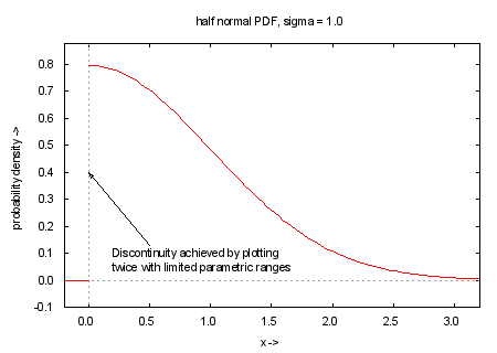
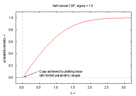
set title "half normal PDF, sigma = 1.0"
set arrow 1 from 0.5,0.13 to 0.0,0.4
set label 1 "Discontinuity achieved by plotting\ntwice with limited parametric ranges" at 0.2,0.1 left
plot t<0?t:-eps, halfnormal(t<0?t:-eps, sigma) ls 1, t<0?0.0:t, halfnormal(t<0?0.0:t, sigma) ls 1

Click here for minimal script to generate this plot

set title "half normal CDF, sigma = 1.0"
set yrange [-0.1:1.1]
set arrow 1 from 0.45,0.1 to 0.05,0.01
set label 1 "Cusp achieved by plotting twice\nwith limited parametric ranges" at 0.5,0.1 left
plot t<0?t:-eps, chalfnormal(t<0?t:-eps, sigma) ls 1, t<0?0.0:t, chalfnormal(t<0?0.0:t, sigma) ls 1

Click here for minimal script to generate this plot

unset label 1
unset arrow 1
unset parametric

# Hypergeometric PDF and CPF
N = 75; C = 25; d = 10
p = real(C) / N
mu = d * p
sigma = sqrt(real(N - d) / (N - 1.0) * d * p * (1.0 - p))
xmin = int(mu - 4.0 * sigma)
xmin = xmin < -1 ? -1 : xmin
xmax = int(mu + 4.0 * sigma)
xmax = xmax < d+1 ? d+1 : xmax
ymax = 1.1 * hypgeo(int(mu),N,C,d) # approximate mode of hypergeometric PDF used
unset key
unset zeroaxis
set xrange [xmin : xmax]
set yrange [0 : ymax]
set xlabel "k ->"
set ylabel "probability density ->"
set ytics 0, ymax / 10, ymax
set format x "%2.0f"
set format y "%3.2f"
set sample (xmax - xmin) + 1
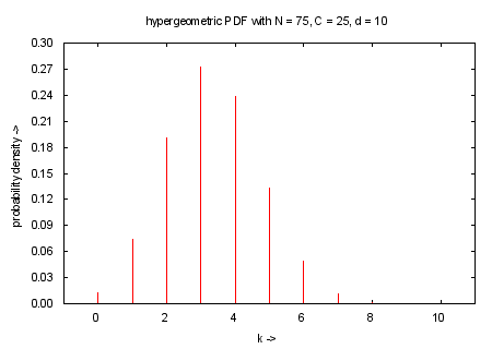
set title "hypergeometric PDF with N = 75, C = 25, d = 10"
plot hypgeo(x,N,C,d) with impulses

Click here for minimal script to generate this plot

set yrange [0 : 1.1]
set ytics 0, 1.0 / 10.0, 1.1
set title "hypergeometric CDF with N = 75, C = 25, d = 10"
plot chypgeo(x,N,C,d) with steps

Click here for minimal script to generate this plot

# Laplace PDF
mu = 0.0; b = 1.0
sigma = sqrt(2.0) * b
xmin = mu - 4.0 * sigma
xmax = mu + 4.0 * sigma
ymax = 1.1 * laplace(mu, mu, b) #Mode of laplace PDF used
unset key
set zeroaxis
set xrange [xmin: xmax]
set yrange [0: ymax]
set xlabel "x ->"
set ylabel "probability density ->"
set xtics autofreq
set ytics autofreq
set format x "%.1f"
set format y "%.2f"
set sample 100+1
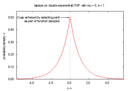
set title "laplace (or double exponential) PDF with mu = 0, b = 1"
set arrow 1 from -0.95,0.5 to -0.1,0.5
set label 1 "Cusp achieved by selecting point\nas part of function samples" at -1.0,0.5 right
plot laplace(x, mu, b)

Click here for minimal script to generate this plot

unset label 1
unset arrow 1
set title "laplace (or double exponential) CDF with mu = 0, b = 1"
set yrange [0: 1.1]
plot claplace(x, mu, b)

Click here for minimal script to generate this plot

# Logistic PDF and CDF
a = 0.0; lambda = 2.0
mu = a
sigma = pi / (sqrt(3.0) * lambda)
xmin = mu - 4.0 * sigma
xmax = mu + 4.0 * sigma
ymax = 1.1 * logistic(mu, a, lambda) #Mode of logistic PDF used
unset key
set zeroaxis
set xrange [xmin: xmax]
set yrange [0: ymax]
unset key
set zeroaxis
set xlabel "x ->"
set ylabel "probability density ->"
set xtics autofreq
set ytics autofreq
set format x "%.1f"
set format y "%.1f"
set sample 100
set title "logistic PDF with a = 0, lambda = 2"
plot logistic(x, a, lambda)

Click here for minimal script to generate this plot

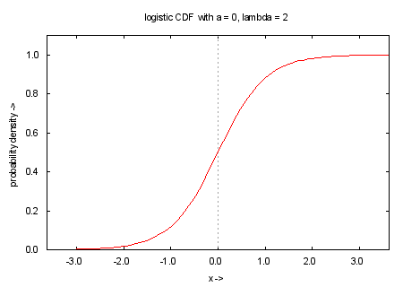
set title "logistic CDF with a = 0, lambda = 2"
set yrange [0: 1.1]
plot clogistic(x, a, lambda)

Click here for minimal script to generate this plot

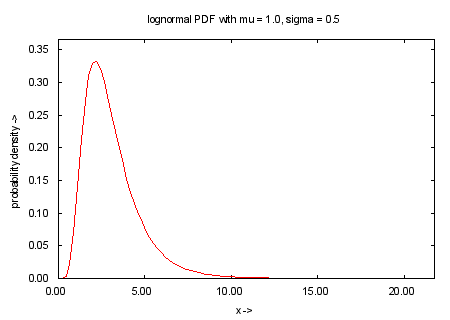
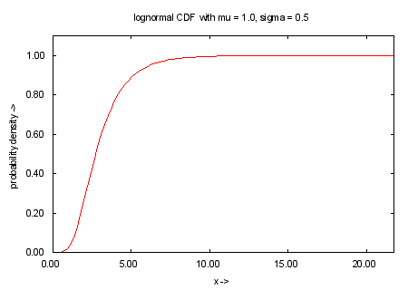
# Lognormal PDF and CDF
mu = 1.0; sigma = 0.5
m = exp(mu + 0.5 * sigma**2)
s = sqrt(exp(2.0 * mu + sigma**2) * (2.0 * exp(sigma) - 1.0))
xmin = m - 4.0 * s
xmin = xmin < 0 ? 0 : xmin
xmax = m + 4.0 * s
ymax = 1.1 * lognormal(exp(mu - sigma**2), mu, sigma) #Mode of lognormal PDF used
unset key
set zeroaxis
set xrange [xmin: xmax]
set yrange [0: ymax]
set xlabel "x ->"
set ylabel "probability density ->"
set xtics autofreq
set ytics autofreq
set format x "%.2f"
set format y "%.2f"
set sample 100
set title "lognormal PDF with mu = 1.0, sigma = 0.5"
plot lognormal(x, mu, sigma)

Click here for minimal script to generate this plot

set title "lognormal CDF with mu = 1.0, sigma = 0.5"
set yrange [0: 1.1]
plot clognormal(x, mu, sigma)

Click here for minimal script to generate this plot

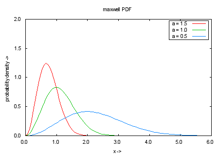
# Maxwell PDF
a = 0.5
mu = 2.0 / sqrt(pi) / a
sigma = sqrt(3.0 - 8.0/pi) / a
xmin = int(mu - 3.0 * sigma)
xmin = xmin < 0 ? 0 : xmin
xmax = int(mu + 3.0 * sigma)
a = 1.5
ymax = 1.1 * maxwell(1.0 / a, a) + 0.5 #Mode of maxwell PDF used
ymax = int(ymax + 0.5)
set zeroaxis
set xlabel "x ->"
set ylabel "probability density ->"
set xtics autofreq
set ytics autofreq
set format x "%.1f"
set format y "%.1f"
set sample 100
set title "maxwell PDF"
set key right top box
plot [xmin:xmax] [0:ymax] maxwell(x, 1.5) title "a = 1.5", \
                   maxwell(x, 1.0) title "a = 1.0", \
                   maxwell(x, 0.5) title "a = 0.5"

Click here for minimal script to generate this plot

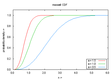
set title "maxwell CDF"
set key right bottom box
plot [xmin:xmax] [0:1.1] cmaxwell(x, 1.5) title "a = 1.5", \
                         cmaxwell(x, 1.0) title "a = 1.0", \
                         cmaxwell(x, 0.5) title "a = 0.5"

Click here for minimal script to generate this plot

# Negative binomial PDF and CDF
r = 8; p = 0.4
mu = r * (1.0 - p) / p
sigma = sqrt(mu / p)
xmin = int(mu - 4.0 * sigma)
xmin = xmin < 0 ? 0 : xmin
xmax = int(mu + 4.0 * sigma)
ymax = 1.1 * negbin(int(mu - (1.0-p)/p), r, p) #mode of gamma PDF used
unset key
unset zeroaxis
set xrange [xmin-1 : xmax]
set yrange [0 : ymax]
set xlabel "k ->"
set ylabel "probability density ->"
set ytics 0, ymax / 10, ymax
set format x "%2.0f"
set format y "%3.2f"
set sample (xmax - xmin+1) + 1
set title "negative binomial (or pascal or polya) PDF with r = 8, p = 0.4"
plot negbin(x, r, p) with impulses

Click here for minimal script to generate this plot

set yrange [0 : 1.1]
set ytics 0, 0.1, 1.0
set title "negative binomial (or pascal or polya) CDF with r = 8, p = 0.4"
plot cnegbin(x, r, p) with steps

Click here for minimal script to generate this plot

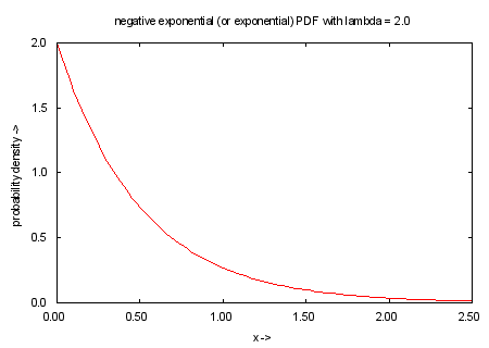
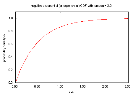
# Negative exponential PDF and CDF
lambda = 2.0
mu = 1.0 / lambda
sigma = 1.0 / lambda
xmax =  mu + 4.0 * sigma
ymax = lambda #No mode
unset key
set zeroaxis
set xrange [0: xmax]
set yrange [0: ymax]
set xlabel "x ->"
set ylabel "probability density ->"
set xtics autofreq
set ytics autofreq
set format x "%.2f"
set format y "%.1f"
set sample 100
set title "negative exponential (or exponential) PDF with lambda = 2.0"
plot nexp(x, lambda)

Click here for minimal script to generate this plot

set title "negative exponential (or exponential) CDF with lambda = 2.0"
set yrange [0: 1.1]
plot cnexp(x, lambda)

Click here for minimal script to generate this plot

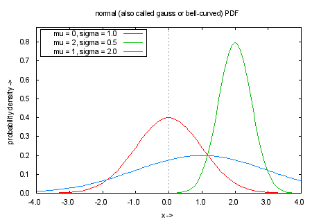
# Normal PDF and CDF
mu = 0.0; sigma = 1.0
xmin = mu - 4.0 * sigma
xmax = mu + 4.0 * sigma
mu = 2.0; sigma = 0.5
ymax = 1.1 * normal(mu, mu, sigma) #Mode of normal PDF used
set zeroaxis
set xlabel "x ->"
set ylabel "probability density ->"
set xtics autofreq
set ytics autofreq
set format x "%.1f"
set format y "%.1f"
set sample 100
set title "normal (also called gauss or bell-curved) PDF"
set key left top box
plot [xmin:xmax] [0:ymax] normal(x, 0, 1.0) title "mu = 0, sigma = 1.0", \
                          normal(x, 2, 0.5) title "mu = 2, sigma = 0.5", \
                          normal(x, 1, 2.0) title "mu = 1, sigma = 2.0"

Click here for minimal script to generate this plot

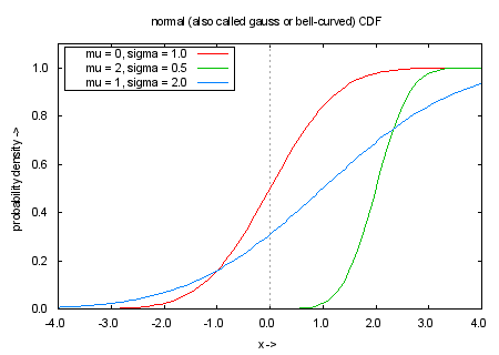
set title "normal (also called gauss or bell-curved) CDF"
set key left top box
plot [xmin:xmax] [0:1.1] mu = 0, sigma = 1.0, cnormal(x, mu, sigma) title "mu = 0, sigma = 1.0", \
                         mu = 2, sigma = 0.5, cnormal(x, mu, sigma) title "mu = 2, sigma = 0.5", \
                         mu = 1, sigma = 2.0, cnormal(x, mu, sigma) title "mu = 1, sigma = 2.0"

Click here for minimal script to generate this plot

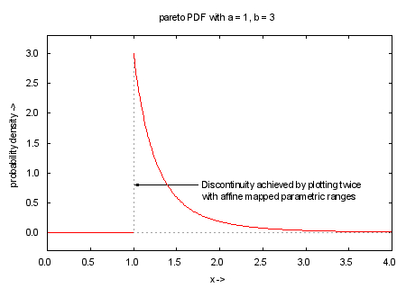
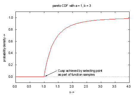
# Pareto PDF and CDF
a = 1.0; b = 3.0
mu = a * b / (b - 1.0)
sigma = a * sqrt(b) / (sqrt(b - 2.0) * (b - 1.0))
xmin = mu - 4.0 * sigma
xmin = xmin < 0 ? 0 : xmin
xmax = int(mu + 4.0 * sigma)
ymax = 1.1 * pareto(a, a, b) #mode of pareto PDF used
ymin = -0.1 * pareto(a, a, b)
unset key
set zeroaxis
set xrange [xmin: xmax]
set yrange [ymin: ymax]
set xlabel "x ->"
set ylabel "probability density ->"
set xtics autofreq
set ytics autofreq
set format x "%.1f"
set format y "%.1f"
set sample 200+1
set title "pareto PDF with a = 1, b = 3"
# Discontinuity at a
set parametric
set trange [0:1-eps]
x1(t) = -1 + 2*t
x2(t) =  1 + 3*t
set arrow 1 from 1.75,0.8 to 1.0,0.8
set arrow 2 from 1.0,0.0 to 1.0,3.0 nohead lt 0
set label 1 "Discontinuity achieved by plotting twice\nwith affine mapped parametric ranges" at 1.8,0.8 left
plot x1(t), pareto(x1(t), a, b) ls 1, x2(t), pareto(x2(t), a, b) ls 1

Click here for minimal script to generate this plot

unset arrow 2
set title "pareto CDF with a = 1, b = 3"
unset parametric
set yrange [-0.1: 1.1]
set arrow 1 from 1.45,0.1 to 1.05,0.01
set label 1 "Cusp achieved by selecting point\nas part of function samples" at 1.5,0.1 left
plot cpareto(x, a, b)

Click here for minimal script to generate this plot

unset label 1
unset arrow 1

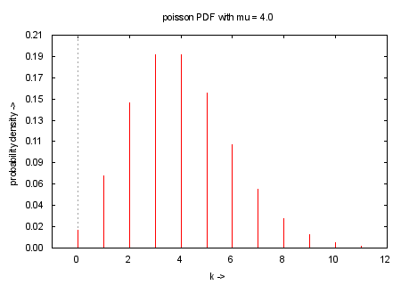
# Poisson PDF and CDF
mu = 4.0
sigma = sqrt(mu)
xmin = int(mu - 4.0 * sigma)
xmin = xmin < -1 ? -1 : xmin
xmax = int(mu + 4.0 * sigma)
ymax = 1.1 * poisson(mu, mu) #mode of poisson PDF used
unset key
set zeroaxis
set xrange [xmin : xmax]
set yrange [0 : ymax]
set xlabel "k ->"
set ylabel "probability density ->"
set ytics 0, ymax / 10, ymax
set format x "%2.0f"
set format y "%3.2f"
set sample (xmax - xmin) + 1
set title "poisson PDF with mu = 4.0"
plot poisson(x, mu) with impulses

Click here for minimal script to generate this plot

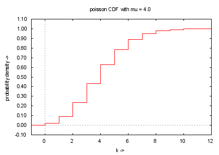
set yrange [-0.1 : 1.1]
set ytics -0.1, 0.1, 1.1
set title "poisson CDF with mu = 4.0"
plot cpoisson(x, mu) with steps

Click here for minimal script to generate this plot

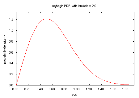
# Rayleigh PDF and CDF
lambda = 2.0
mu = 0.5 * sqrt(pi / lambda)
sigma = sqrt((1.0 - pi / 4.0) / lambda)
xmax = mu + 4.0 * sigma
ymax = 1.1 * rayleigh(1.0 / sqrt(2.0 * lambda), lambda) #Mode of rayleigh PDF used
unset key
set zeroaxis
set xrange [0: xmax]
set yrange [0: ymax]
set xlabel "x ->"
set ylabel "probability density ->"
set xtics autofreq
set ytics autofreq
set format x "%.2f"
set format y "%.1f"
set sample 100
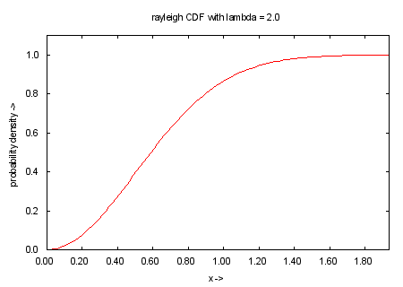
set title "rayleigh PDF with lambda = 2.0"
plot rayleigh(x, lambda)

Click here for minimal script to generate this plot

set title "rayleigh CDF with lambda = 2.0"
set yrange [0: 1.1]
plot crayleigh(x, lambda)

Click here for minimal script to generate this plot

# Sine PDF and CDF
a = 3.2; f = 2.6
mu = a / 2.0
sigma = sqrt(a * a / 3.0 * (1.0 - 3.0 / (2.0 * n * n * pi * pi)) - mu * mu)
xmin = 0.0
xmax = a - eps
a = 2; f = 1.0
ymax = 1.1 * 2.0 / a #Mode of sine PDF used
set zeroaxis
set xlabel "x ->"
set ylabel "probability density ->"
set xtics autofreq
set ytics autofreq
set format x "%.2f"
set format y "%.1f"
set sample 250
set title "sine PDF"
set key bottom outside
keystr(a, f) = sprintf("a = %0.1f, f = %0.1f", a, f)
a1 = 2.0; a2 = 3.25; a3 = 2.75
f1 = 1.0; f2 = 3.0; f3 = 2.6; f4 = 0.0
plot [xmin:xmax] [0:ymax] a = a1, f = f1, sine(x, f, a) title keystr(a, f), \
                          a = a1, f = f2, sine(x, f, a) title keystr(a, f), \
                          a = a2, f = f3, sine(x, f, a) title keystr(a, f), \
                          a = a3, f = f4, sine(x, f, a) title keystr(a, f) with steps

Click here for minimal script to generate this plot

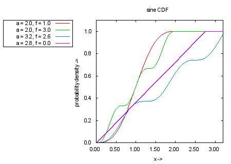
set title "sine CDF"
set key top left
plot [xmin:xmax] [0:1.1] a = a1, f = f1, csine(x, f, a) title keystr(a, f), \
                         a = a1, f = f2, csine(x, f, a) title keystr(a, f), \
                         a = a2, f = f3, csine(x, f, a) title keystr(a, f), \
                         a = a3, f = f4, csine(x, f, a) title keystr(a, f) with steps

Click here for minimal script to generate this plot

# t PDF and CDF
nu = 20
mu = 0
sigma = nu > 2 ? sqrt(nu / (nu - 2.0)) : 1.0
xmin = mu - 4.0 * sigma
xmax = mu + 4.0 * sigma
ymax = 1.1 * t(mu, nu) #Mode of t PDF used
set key inside center left title "degrees of freedom"
set zeroaxis
set xrange [xmin: xmax]
set yrange [0: ymax]
set xlabel "x ->"
set ylabel "probability density ->"
set xtics autofreq
set ytics autofreq
set format x "%.1f"
set format y "%.2f"
set sample 100
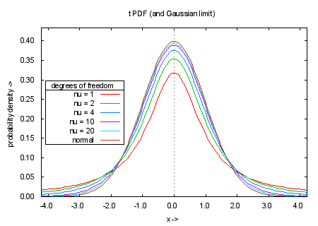
set title "t PDF (and Gaussian limit)"
ks(nu) = sprintf("nu = %d", nu)
plot t(x, 1) ti ks(1), t(x, 2) ti ks(2), t(x, 4) ti ks(4), t(x, 10) ti ks(10), \
     t(x, 20) ti ks(20), normal(x, 0, 1) ti "normal"

Click here for minimal script to generate this plot

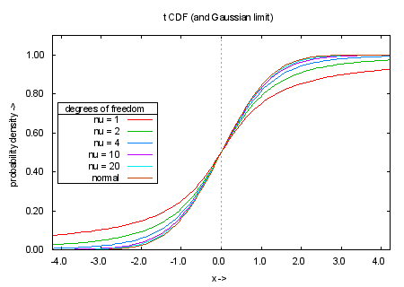
set title "t CDF (and Gaussian limit)"
set yrange [0: 1.1]
plot ct(x, 1) ti ks(1), ct(x, 2) ti ks(2), ct(x, 4) ti ks(4), ct(x, 10) ti ks(10), \
     ct(x, 20) ti ks(20), cnormal(x, 0, 1) ti "normal"

Click here for minimal script to generate this plot

# Thanks to efrank@upenn5.hep.upenn.edu for telling us about this
# triangular PDF and CDF
m = 3.0
g = 2.0
mu = m
sigma = g/sqrt(6.0)
xmin = m - 1.1*g
xmax = m + 1.1*g
ymax = 1.1 * triangular(m, m, g) #Mode of triangular PDF used
ymin = -ymax/11.0;
unset key
set zeroaxis
set xrange [xmin: xmax]
set yrange [ymin: ymax]
set xlabel "x ->"
set ylabel "probability density ->"
set xtics autofreq
set ytics autofreq
set format x "%.1f"
set format y "%.2f"
set sample 50*1.1*g+1
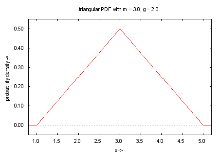
set title "triangular PDF with m = 3.0, g = 2.0"
plot triangular(x, m, g)

Click here for minimal script to generate this plot

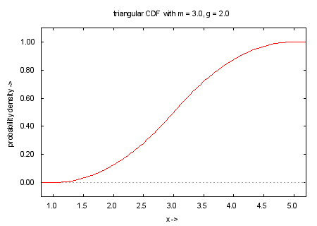
set title "triangular CDF with m = 3.0, g = 2.0"
set yrange [-0.1: 1.1]
plot ctriangular(x, m, g)

Click here for minimal script to generate this plot

# Uniform PDF and CDF
a = -2.0; b= 2.0
mu = (a + b) / 2.0
sigma = (b - a) / sqrt(12.0)
xmin = a - 0.1*(b - a)
xmax = b + 0.1*(b - a)
ymax = 1.1 * uniform(mu, a, b) #No mode
ymin = -0.1 * uniform(mu, a, b)
unset key
set zeroaxis
set xrange [xmin: xmax]
set yrange [ymin: ymax]
set xlabel "x ->"
set ylabel "probability density ->"
set xtics autofreq
set ytics autofreq
set format x "%.2f"
set format y "%.2f"
set sample 120+1
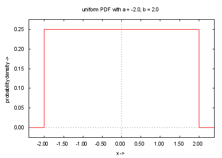
set title "uniform PDF with a = -2.0, b = 2.0"
plot uniform(x, a, b) with steps

Click here for minimal script to generate this plot

set title "uniform CDF with a = -2.0, b = 2.0"
set yrange [-0.1 : 1.1]
plot cuniform(x, a, b)

Click here for minimal script to generate this plot

# Weibull PDF and CDF
lambda = 1.0/5; a = 1.0
mu = 1.0 / lambda * gamma(1.0 / a) / a
sigma = sqrt(lambda**(-2.0) * (2.0 * gamma(2.0 / a) / a - (gamma(1.0 / a) / a)**2))
xmin = mu - 4.0 * sigma
xmin = xmin < 0 ? 0 : xmin
#Mode of weibull PDF used
ymax = 1.8 * (a >= 1.0 ? weibull(((a - 1.0) / a)**(1.0 / a) / lambda, a, lambda) : 2.0)
lambda = 1.0/15; a = 10.0
mu = 1.0 / lambda * gamma(1.0 / a) / a
sigma = sqrt(lambda**(-2.0) * (2.0 * gamma(2.0 / a) / a - (gamma(1.0 / a) / a)**2))
xmax = int(mu + 4.0 * sigma)
set key on title "" inside top right
set zeroaxis
set grid
set xrange [xmin : xmax]
set xlabel "x ->"
set ylabel "probability density ->"
set xtics autofreq
set ytics autofreq
set format x "%g"
set format y "%g"
set sample 100
set title "weibull PDF"
ks(a,lambda) = sprintf("lambda = 1/%g, a = %0.1f", 1.0/lambda, a)
a1 = 0.5; a2 = 1.0; a3 = 2.0; a4 = 10.0
lambda1 = 1.0/5; lambda2 = 1.0/15
set arrow 1 from 3.8,0.27 to 0.5,weibull(0.5,a1,lambda1)
set label 1 "a < 1, rate descreasing over time" at 4,0.27 left
set arrow 2 from 8,0.19 to 6.4,weibull(6.4,a3,lambda1)
set arrow 3 from 10.5,0.19 to 13,weibull(13,a4,lambda2)
set label 2 "a > 1, rate increasing over time" at 9,0.2 center
plot [] [0:ymax] lambda = lambda1, a = a1, weibull(x, a, lambda) ti ks(a, lambda), \
                 lambda = lambda1, a = a2, weibull(x, a, lambda) ti ks(a, lambda), \
                 lambda = lambda1, a = a3, weibull(x, a, lambda) ti ks(a, lambda), \
                 lambda = lambda2, a = a4, weibull(x, a, lambda) ti ks(a, lambda)

Click here for minimal script to generate this plot

unset label 1; unset label 2
unset arrow 1; unset arrow 2; unset arrow 3
set key at 9,0.4 center
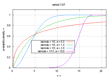
set title "weibull CDF"
plot [] [0:1.1] lambda = lambda1, a = a1, cweibull(x, a, lambda) ti ks(a, lambda), \
                lambda = lambda1, a = a2, cweibull(x, a, lambda) ti ks(a, lambda), \
                lambda = lambda1, a = a3, cweibull(x, a, lambda) ti ks(a, lambda), \
                lambda = lambda2, a = a4, cweibull(x, a, lambda) ti ks(a, lambda)

Click here for minimal script to generate this plot