|
set title "\"fence plot\" using separate parametric surfaces"
# A method suggested by Hans-Bernhard Broeker
# <broeker@physik.rwth-aachen.de>: display a separate parametric
# surface for each fence.
set zrange [-1:1]
unset label
unset arrow
set xrange [-5:5]; set yrange [-5:5]
set arrow from 5,-5,-1.2 to 5,5,-1.2 lt -1
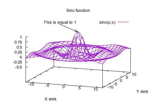
set label 1 "increasing v" at 6,0,-1
set arrow from 5,6,-1 to 5,5,-1 lt -1
set label 2 "u=0" at 5,6.5,-1
set arrow from 5,6,sinc(5,5) to 5,5,sinc(5,5) lt -1
set label 3 "u=1" at 5,6.5,sinc(5,5)
set parametric
set hidden3d
set isosamples 2,33
xx=-5; dx=(4.99-(-4.99))/9
x0=xx; xx=xx+dx
x1=xx; xx=xx+dx
x2=xx; xx=xx+dx
x3=xx; xx=xx+dx
x4=xx; xx=xx+dx
x5=xx; xx=xx+dx
x6=xx; xx=xx+dx
x7=xx; xx=xx+dx
x8=xx; xx=xx+dx
x9=xx; xx=xx+dx
splot [u=0:1][v=-4.99:4.99] \
x0, v, (u<0.5) ? -1 : sinc(x0,v) notitle, \
x1, v, (u<0.5) ? -1 : sinc(x1,v) notitle, \
x2, v, (u<0.5) ? -1 : sinc(x2,v) notitle, \
x3, v, (u<0.5) ? -1 : sinc(x3,v) notitle, \
x4, v, (u<0.5) ? -1 : sinc(x4,v) notitle, \
x5, v, (u<0.5) ? -1 : sinc(x5,v) notitle, \
x6, v, (u<0.5) ? -1 : sinc(x6,v) notitle, \
x7, v, (u<0.5) ? -1 : sinc(x7,v) notitle, \
x8, v, (u<0.5) ? -1 : sinc(x8,v) notitle, \
x9, v, (u<0.5) ? -1 : sinc(x9,v) notitle
Click here for minimal script to generate this plot
|