Back to demo index

gnuplot demo script: bivariat.dem

autogenerated by webify.pl on Fri Oct 28 21:04:51 2016
gnuplot version gnuplot 5.0 patchlevel 5
#
# $Id: bivariat.dem,v 1.9 2011/08/01 05:14:23 sfeam Exp $
#
# This demo is very slow and requires unusually large stack size.
# Do not attempt to run this demo under MSDOS.
#

# the function integral_f(x) approximates the integral of f(x) from 0 to x.
# integral2_f(x,y) approximates the integral from x to y.
# define f(x) to be any single variable function
#
# the integral is calculated using Simpson's rule as 
#          ( f(x-delta) + 4*f(x-delta/2) + f(x) )*delta/6
# repeated x/delta times (from x down to 0)
#
delta = 0.2
#  delta can be set to 0.025 for non-MSDOS machines
#
# integral_f(x) takes one variable, the upper limit.  0 is the lower limit.
# calculate the integral of function f(t) from 0 to x
# choose a step size no larger than delta such that an integral number of
# steps will cover the range of integration.
integral_f(x) = (x>0)?int1a(x,x/ceil(x/delta)):-int1b(x,-x/ceil(-x/delta))
int1a(x,d) = (x<=d*.1) ? 0 : (int1a(x-d,d)+(f(x-d)+4*f(x-d*.5)+f(x))*d/6.)
int1b(x,d) = (x>=-d*.1) ? 0 : (int1b(x+d,d)+(f(x+d)+4*f(x+d*.5)+f(x))*d/6.)
#
# integral2_f(x,y) takes two variables; x is the lower limit, and y the upper.
# calculate the integral of function f(t) from x to y
integral2_f(x,y) = (x<y)?int2(x,y,(y-x)/ceil((y-x)/delta)): \
                        -int2(y,x,(x-y)/ceil((x-y)/delta))
int2(x,y,d) = (x>y-d*.5) ? 0 : (int2(x+d,y,d) + (f(x)+4*f(x+d*.5)+f(x+d))*d/6.)

set autoscale
set title "approximate the integral of functions"
set samples 50
set key bottom right

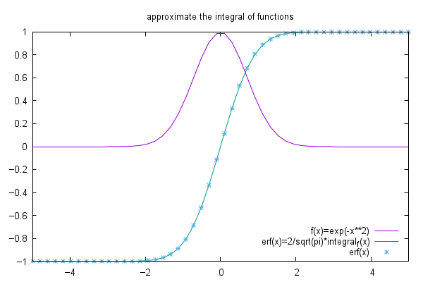
f(x) = exp(-x**2)

plot [-5:5] f(x) title "f(x)=exp(-x**2)", \
  2/sqrt(pi)*integral_f(x) title "erf(x)=2/sqrt(pi)*integral_f(x)", \
  erf(x) with points


Click here for minimal script to generate this plot
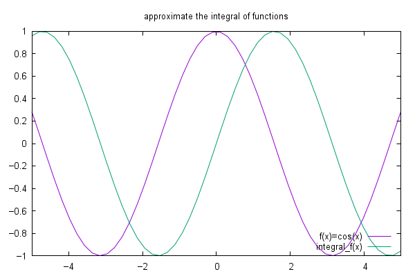


f(x)=cos(x)

plot [-5:5] f(x) title "f(x)=cos(x)", integral_f(x)


Click here for minimal script to generate this plot
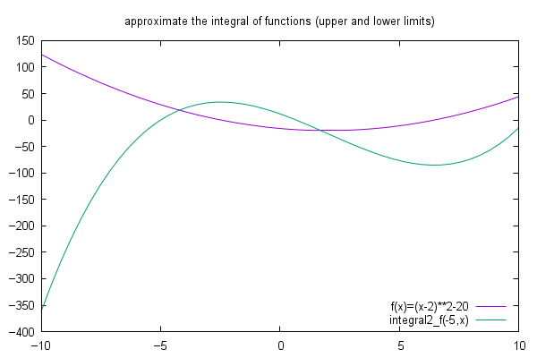


set title "approximate the integral of functions (upper and lower limits)"

f(x)=(x-2)**2-20

plot [-10:10] f(x) title "f(x)=(x-2)**2-20", integral2_f(-5,x)


Click here for minimal script to generate this plot
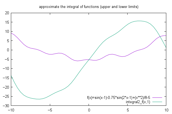


f(x)=sin(x-1)-.75*sin(2*x-1)+(x**2)/8-5

plot  [-10:10] f(x) title "f(x)=sin(x-1)-0.75*sin(2*x-1)+(x**2)/8-5", integral2_f(x,1)


Click here for minimal script to generate this plot


#
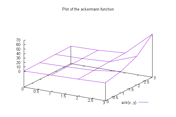
# This definition computes the ackermann. Do not attempt to compute its
# values for non integral values. In addition, do not attempt to compute
# its beyond m = 3, unless you want to wait really long time.

ack(m,n) = (m == 0) ? n + 1 : (n == 0) ? ack(m-1,1) : ack(m-1,ack(m,n-1))

set xrange [0:3]
set yrange [0:3]

set isosamples 4
set samples 4

set title "Plot of the ackermann function"

splot ack(x, y)


Click here for minimal script to generate this plot
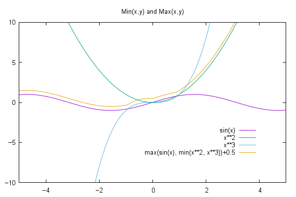


set xrange [-5:5]
set yrange [-10:10]
set isosamples 10
set samples 100
set key top right at 4,-3
set title "Min(x,y) and Max(x,y)"

#
min(x,y) = (x < y) ? x : y
max(x,y) = (x > y) ? x : y

plot sin(x), x**2, x**3, max(sin(x), min(x**2, x**3))+0.5


Click here for minimal script to generate this plot


#
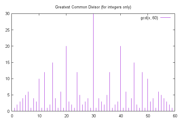
# gcd(x,y) finds the greatest common divisor of x and y,
#          using Euclid's algorithm
# as this is defined only for integers, first round to the nearest integer
gcd(x,y) = gcd1(rnd(max(x,y)),rnd(min(x,y)))
gcd1(x,y) = (y == 0) ? x : gcd1(y, x - x/y * y)
rnd(x) = int(x+0.5)

set samples 59
set xrange [1:59]
set auto
set key default

set title "Greatest Common Divisor (for integers only)"

plot gcd(x, 60) with impulses

Click here for minimal script to generate this plot


#
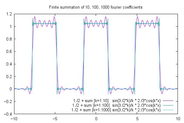
# This definition computes the sum of the first 10, 100, 1000 fourier
# coefficients of a (particular) square wave.

set title "Finite summation of 10, 100, 1000 fourier coefficients"

set samples 500
set xrange [-10:10]
set yrange [-0.4:1.2]
set key bottom right

fourier(k, x) = sin(3./2*k)/k * 2./3*cos(k*x)
sum10(x)   = 1./2 + sum [k=1:10]   fourier(k, x)
sum100(x)  = 1./2 + sum [k=1:100]  fourier(k, x)
sum1000(x) = 1./2 + sum [k=1:1000] fourier(k, x)

plot \
    sum10(x)   title "1./2 + sum [k=1:10]   sin(3./2*k)/k * 2./3*cos(k*x)", \
    sum100(x)  title "1./2 + sum [k=1:100]  sin(3./2*k)/k * 2./3*cos(k*x)", \
    sum1000(x) title "1./2 + sum [k=1:1000] sin(3./2*k)/k * 2./3*cos(k*x)"

Click here for minimal script to generate this plot