#
# $Id: random.dem,v 1.16 2014/03/23 13:27:27 markisch Exp $
#
# random.dem
#
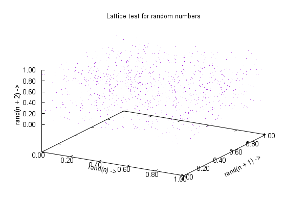
# Lattice test for random numbers;
# If you can see any patterns in this plot, the random number generator
# is not very good.
#
# Copyright (c) 1991, Jos van der Woude, jvdwoude@hut.nl

# History:
#	-  6. 6. 2006 ds: added univariate and multivariate normal example
#	- 10. 5. 2006 ds: added univariate and multivariate normal example
#	-  ?. ?  1991 jvdw: 1st version

unset key
set xrange [0: 1]
set yrange [0: 1]
set zrange [0: 1]
set title "Lattice test for random numbers"
set xlabel "rand(n) ->"      rotate parallel
set ylabel "rand(n + 1) ->"  rotate parallel offset 0,-1
set zlabel "rand(n + 2) ->"  rotate parallel offset 0,-1
set format x "%3.2f"
set format y "%3.2f"
set format z "%3.2f"
set tics
set sample 1000
set style function dots
set parametric
plot rand(0), rand(0)

Click here for minimal script to generate this plot

print "3D plot ahead, one moment please ..."
set sample 50
splot rand(0), rand(0), rand(0)

Click here for minimal script to generate this plot

print ""
print "Multivariate normal distribution"
print ""
print "The surface plot shows a two variable multivariate probability"
print "density function.  On the x-y plane are some samples of the random"
print "vector and a contour plot illustrating the correlation, which in"
print "this case is zero, i.e. a circle.  (Easier to view in map mode.)"
print ""
nsamp = 50
# Generate N random data points.
set print $random
do for [i=1:nsamp] {
    print sprintf("%8.5g %8.5g", invnorm(rand(0)), invnorm(rand(0)))
}
unset print
#
unset xlabel
unset ylabel
unset zlabel
set parametric
tstring(n) = sprintf("%d random samples from a 2D Gaussian PDF with\nunit variance, zero mean and no dependence", n)
set title tstring(nsamp)
unset key
set hidden3d
set contour
set view 68, 28, 1, 1
set cntrparam levels discrete 0.1
unset clabel
set xrange [-3:3]
set yrange [-3:3]
set zrange [-0.2:0.2]
set ztics 0,0.05
set urange [-3:3]
set vrange [-3:3]
set ticslevel 0
set isosamples 30
splot u,v,( 1/(2*pi) * exp(-0.5 * (u**2 + v**2)) ) with line lc rgb "black", \
   $random using 1:2:(-0.2) with points pointtype 7 lc rgb "black"

Click here for minimal script to generate this plot

unset contour
unset parametric

load "stat.inc"

print ""
print "Simple Monte Carlo simulation"
print ""
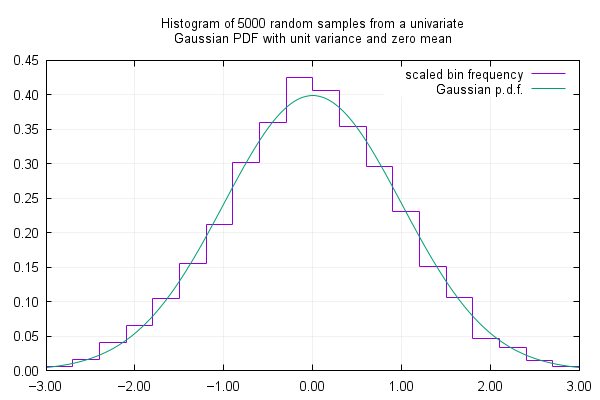
print "The first curve is a histogram where the binned frequency of occurrence"
print "of a pseudo random variable distributed according to the normal"
print "(Gaussian) law is scaled such that the histogram converges to the"
print "normal probability density function with increasing number of samples"
print "used in the Monte Carlo simulation.  The second curve is the normal"
print "probability density function with unit variance and zero mean."
print ""
nsamp = 5000
binwidth = 20
xlow = -3.0
xhigh = 3.0
scale = (binwidth/(xhigh-xlow))
# Generate N random data points.
set print $random
do for [i=1:nsamp] {
    print sprintf("%8.5g %8.5g", invnorm(rand(0)), (1.0*scale/nsamp))
}
unset print
#
set samples 200
tstring(n) = sprintf("Histogram of %d random samples from a univariate\nGaussian PDF with unit variance and zero mean", n)
set title tstring(nsamp)
set key
set grid
set xrange [-3:3]
set yrange [0:0.45]
bin(x) = (1.0/scale)*floor(x*scale)
plot $random using (bin($1)):2 smooth frequency with steps \
                title "scaled bin frequency", \
                normal(x,0,1) with lines title "Gaussian p.d.f."

Click here for minimal script to generate this plot

print ""
print "Another Monte Carlo simulation"
print ""
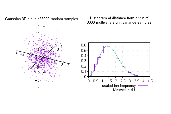
print "This is similar to the previous simulation but uses multivariate"
print "zero mean, unit variance normal data by computing the distance "
print "each point is from the origin.  That distribution is known to fit"
print "the Maxwell probability law, as shown."
print ""
undefine $random
load "gen-random.inc"
#
oneplot = 1
#
if (oneplot) set multiplot layout 1,2
#
unset key
rlow = -4.0
rhigh = 4.0
set parametric
set xrange [rlow:rhigh]; set yrange [rlow:rhigh]; set zrange [rlow:rhigh]
set xtics axis nomirror; set ytics axis nomirror; set ztics axis nomirror;
set border 0
set xyplane at 0
set xzeroaxis lt -1
set yzeroaxis lt -1
set zzeroaxis lt -1
set view 68, 28, 1.4, 0.9
tstring(n) = sprintf("Gaussian 3D cloud of %d random samples\n", n)
set title tstring(nsamp) offset graph 0.15, graph -0.33
splot $random every :::::0 with dots
if (!oneplot) pause -1 "Hit return to continue"

unset parametric
unset xzeroaxis; unset yzeroaxis;
set border
set grid
set samples 200
set size 0.47,0.72
set origin 0.44,0.18
tstring(n) = sprintf("Histogram of distance from origin of\n%d multivariate unit variance samples", n)
set title tstring(nsamp) offset graph 0, graph 0.15
set key bmargin right vertical
xlow = 0.0
xhigh = 4.5
binwidth = 20
scale = (binwidth/(xhigh-xlow))
set xrange [0:xhigh]
set yrange [0:0.65]
bin(x) = (1.0/scale)*floor(x*scale)
plot $random using (bin(sqrt($1**2+$2**2+$3**2))):(1.0*scale/nsamp) every :::::0 smooth frequency with steps \
                title "scaled bin frequency", \
                maxwell(x, 1/sqrt(2)) with lines title "Maxwell p.d.f."
#
if (oneplot) unset multiplot
#

Click here for minimal script to generate this plot